Data Science & Machine Learning - 5 SF Salaries Kaggle

Hi friends,

Welcome to another post under Data Science & Machine Learning. In the previous post, we discussed how to read and write data from and to various sources such as csv files, excel files, etc. using Pandas DataFrames. 

This post however will be different from the other ones in a way that we will not be learning anything new in this post but will be reviewing the concepts we have learnt till now using the SF Salaries Dataset available at the Kaggle website. Download the dataset from this Kaggle link. You will be required to login there in order to download the dataset. Once downloaded, copy and paste the csv file to your Jupyter Notebook. 

Note: All the commands discussed below are run in the Jupyter Notebook environment. See this post on Jupyter Notebook to know about it in detail. 

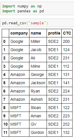
First, import the downloaded Salaries dataset using the read_csv method supported by the Pandas library:

Let's first see a few entries of the SF Salaries Dataset using the head method:

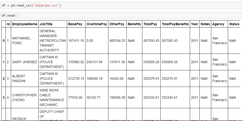
We can see that the dataset has the following columns:

1. Id
2. EmployeeName
3. JobTitle
4. BasePay
5. OvertimePay
6. OtherPay
7. Benefits
8. TotalPay
9. TotalPayBenefits
10. Year
11. Notes
12. Agency
13. Status

We can find the total number of entries in the SF dataset using the info method:

Now, let's answer some relevant questions using the concepts we have gathered till now:

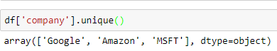
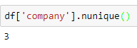
1. Unique Job Titles in the dataset:





2. Top 10 most common Job Titles:





3. Average BasePay of the dataset:





4. Maximum amount of OvertimePay of the dataset:





5. JobTitle of ALBERT PARDINI:





6. TotalPayBenefits of ALBERT PARDINI:





7. Individual with highest TotalPayBenefits in the dataset: 




We can get the above result using the advance argmax method as well:





8. Average TotalPay year-wise:





9. Number of individuals with Chief in their Job Title: This involves lambda expression and might appear tricky at first sight but I suggest to break it down into sub steps for clear understanding. 

It is always advisable to explore various datasets from Kaggle or other websites since Data Science is not about just reading the theory but applying those concepts to datasets and gain insights to achieve a desirable output. From the next posts on ward, we'll start learning about another very important aspect of Data Science i.e. Data Visualizing. 

Read More

Data Science & Machine Learning - 4.7 Pandas Input Output

Hi friends,

Welcome to another post under Data Science & Machine Learning. In the previous post, we discussed various important methods supported by Pandas DataFrames. In this post, we will see another important feature of reading and writing data to and from Pandas DataFrames using various resources.

Note: All the commands discussed below are run in the Jupyter Notebook environment. See this post on Jupyter Notebook to know about it in detail. 

Pandas Input Output

To see the list of sources we can read data from into Pandas DataFrames, we type the pd.read_ in Jupyter Notebook and press Tab key. It shows the list of functions to read data from into the Pandas DataFrames.

Similarly, typing <df_name>.to_ and pressing the Tab key shows the list of functions to write data to various sources from a Pandas DataFrame.

Let's now see the usage of important ones.

1. Using CSV files: 
• The read_csv method is used to read data from csv files. Make sure that the csv file to be read from should be present in the current working directory. In the example below, I have a csv file named sample which I have read using the read_csv method.  





• The to_csv method on the other hand is used to write data to csv files.





2. Using Excel files: 


• The read_excel method is used to read data from Microsoft Excel files. Once again, make sure that the Excel file to be read from should be present in the current working directory. In the example below, I have an excel file named sample2 which I have read using the read_excel method.  





• The to_excel method on the other hand is used to write data from Pandas DataFrames to excel files





3. Using HTML files: 


• We can even read data from a webpage provided it is contained within the table HTML tag. The read_html method is used to read data from tables in a webpage. Here is an example of read_html which reads data from the following Wikipedia URL.  





There are nine tables in the given Wikipedia URL which can be found by checking the length of the df variable





We can view each of them by using the access mechanism as in case of Python Lists. For example, to view a portion of the third table, run the following command in a Jupyter Notebook cell:

We can also load data to a Pandas DataFrame from a sql file but I'll leave it to you guys in case you are interested. In the next post under Data Science & Machine Learning, we will use the concepts we have learnt till now to explore the Kaggle SF Salaries Dataset.

Read More

Data Science & Machine Learning - 4.6 Pandas DataFrames Methods

Hi friends,

In the previous post under Data Science & Machine Learning, we discussed SQL functionalities of groupby, join and so on supported by Pandas DataFrames. In this post, we will see some important methods supported by the Pandas library that can be performed on DataFrames.

Note: All the commands discussed below are run in the Jupyter Notebook environment. See this post on Jupyter Notebook to know about it in detail. 

Pandas DataFrames Methods

Let's create a sample DataFrame to work with.

Here, I have created a sample DataFrame about employee details. 

So, let's now discuss the important methods supported by the Pandas library. 

1. head() - Returns only the top few elements of the DataFrame to get an idea of how the data in the DataFrame looks like





2. unique() - Returns the array of unique elements in a particular DataFrame's column





3. nunique() - Returns the number of unique elements in a particular DataFrame's column





4. value_counts() - Another very  important method that counts the occurrence of each element of a particular DataFrame column





5. apply() - Although we do have methods such as min, max, etc. supported by Pandas to work with DataFrames yet what if we want to apply custom methods to DataFrames? That's when the apply methods comes to the rescue. The apply method helps us apply our own user defined methods to a DataFrames' columns. So, let's see an example of the apply method:





In the above example, suppose we wanted to double the CTC of each employee of the DataFrame. For that, we have first defined our user defined method double and later use it on the CTC column using the apply method.

We can achieve the above result in a single step by using lambda expression as shown below:





6. columns() - Returns the list of column names of the DataFrame





7. sort_values() - Sorts the DataFrame based on a specific column





We can also sort the DataFrame in descending order by setting the ascending parameter to False.

We end this post here but you can refer this link to get the complete list of methods supported by Pandas library. In the next post, we'll see the various ways to input and output data to and from the Pandas DataFrames.

Read More

Data Science & Machine Learning - 4.5 Pandas SQL Functionalities

Hi friends,

In the previous post under the series of posts under Data Science & Machine Learning, we learnt how to fill in the missing values in the Pandas DataFrames. In this post, we will see the SQL functionalities of Groupby, Merge and Join supported by Pandas DataFrames.

Note: All the commands discussed below are run in the Jupyter Notebook environment. See this post on Jupyter Notebook to know about it in detail.

Pandas SQL Functionalities

So, let's begin with the Groupby functionality first. Groupby helps in grouping large data frames by different columns and applying summary functions on each group. Let's go through an example now to understand it better.

In the above example taken from here, we can see that the first table is grouped based on the column state and then various aggregate function like the max(), min() and average() and applied on it.

Let's now go through some examples using Jupyter Notebook. So, let's first create a sample DataFrame.

In the sample DataFrame created above, we have four columns namely, company, name, profile and CTC. Now, if we want to compute the average CTC of employees based on the company column then we would do the following:

We can also find the average CTC based on the profile:

We can also apply other aggregate functions like sum(), standard deviation (std), min(), max(), etc.

Pandas provide a describe() method that lists these basic measures all together: 

Let's now see the concatenate and join operations on DataFrames. Before we can perform the concatenate and join operations, we first need to create a couple of sample DataFrames.

Now, we concatenate these two DataFrames using the concat() method:

Notice that the DataFrames are concatenated along the rows by default. We can concatenate them along the columns as well by setting axis parameter to 1.

We can also merge the two columns based on the SQL notion of join operation using the merge() method by providing the key parameter:

We can also apply advanced SQL operations of joining the DataFrames such as inner join, outer join and so on. You can refer this link in case you are interested. In the next post, we will see the list of useful methods we can apply on DataFrames.

Read More

Data Science & Machine Learning - 4.4 Pandas DataFrames Missing Values

Hi friends,

In the previous couple of posts under Data Science & Machine Learning, we learnt about the Pandas DataFrames. In this post, we will discuss another very important topic in Data Analysis about how to deal with the missing values in Pandas DataFrames.

DataFrames Missing Values

By “missing values”, it simply means values which are NaN or are not present for whatever reason. An example of a dataset with missing values could be a collection of financial time series, where some of the time series might start on different dates. Thus, values prior to the start date would generally be marked as missing.

The reason we cannot ignore the missing values is that some of the most popular and widely used machine learning libraries such as scikit-learn and TensorFlow in Python caution the user about missing values in their datasets. Various machine learning algorithms expect all the input values to be numerical and to hold meaning. Both of the libraries suggest removing rows and/or columns that contain missing values.

So, now that we agree that we need to deal with missing values, let's see various ways to handle missing values in Pandas DataFrames.

Note: All the commands discussed below are run in the Jupyter Notebook environment. See this post on Jupyter Notebook to know about it in detail.

Let's first create a sample DataFrame with some missing values:

Notice that I have used the reindex() method to fill in the DataFrames with some NaN values. 

The easiest of the ways to deal with missing values is to just drop the rows or columns corresponding to the NaN values using the dropna() method:

By default, the axis parameter is set to 0 which means it drops all those rows from the DataFrame which contain NaN values. We can also make the columns drop in place of the rows by setting the axis parameter to 1. 

Notice that I have modified the two elements of column 'two' to prevent the result to be empty. Also, notice that the result contains only column two since it is the only column which has all non-NaN values.

However, the method of dropping the NaN values is not preferred since it results in loss of valid data. Thus, the better way to deal with NaN values is to fill the NaN values with statistical measures of mean, median or some custom value.

Remember to set the inplace parameter to True in order to make the changes permanent on the DataFrame. 

You can refer to this official link to know in detail about various other ways to deal with missing values in Python. In the next post, we will see SQL functionalities of groupby, join, etc. supported by the Pandas DataFrames.

Read More

Data Science & Machine Learning - 4.3.2 Pandas DataFrames

Hi friends,

Welcome to yet another post on Pandas DataFrames. In the previous post under Data Science & Machine Learning, we discussed how to create a DataFrame using the Pandas library and perform basic operations on DataFrames. In this post, we discuss a more detailed usage of Pandas DataFrames for performing Data Analysis tasks. 

Note: All the commands discussed below are run in the Jupyter Notebook environment. See this post on Jupyter Notebook to know about it in detail.

We use the same steps we used in the previous post to create a sample Pandas DataFrame:

Conditional Selection on Pandas DataFrames

Just like we performed Conditional Selection on NumPy Arrays, we will learn to do the same with Pandas DataFrames in this post. Conditional Selection as described earlier allows us to access the elements of a particular data structure (here DataFrames) based on conditions i.e. select only those elements of the data structure for which the condition(s) is met.

So, let's starting working with some examples. So, if we wanted only the non-negative (>=0) elements of our DataFrame, we use Conditional Selection in the following manner:

1. Get the boolean array corresponding to each cell in the DataFrame based on its value





2. Use the extracted boolean values to filter out the negative values

Notice, the negative values are replaced by NaN leaving out only the non-negative values. We can achieve the same task in a single step as well:

We can apply Conditional Selection to individual columns as well. Here is the step to achieve the same:

Notice that the entire row corresponding to 'Y' index has been dropped from the result since the value corresponding to its column 'D' was negative.

Since the result of the above conditional selection is also a DataFrame, we can also select only a subset of columns from the resultant DataFrame. Here is an example selecting only the columns 'A' and 'E' of the resultant DataFrame:

What it is basically doing is first dropping the rows corresponding to which the value of the element is negative in the 'D' column and then selecting the columns 'A' and 'E' from the resultant DataFrame. It might appear intimidating if you are a beginner but you can grasp it better with practice.

We can also supply multiple conditions at the same time as well using the conditional operator & and |:

We can also change the index i.e. the row labels of the DataFrame using the set_index() method. However, there is a constraint with the set_index() method that the new row labels to be set should be one of the existing columns only. So, we first add a column to our DataFrame and use that temporary column to change the index using set_index() method:

Notice that first I have add a temporary column to our DataFrame which is later used to set the new index of our DataFrame.

With this, we end this post here on Conditional Selection on Pandas DataFrames. In the next post, we will learn Data Science techniques on how do we deal with missing values in a Pandas DataFrame.

Read More