Saturday, 21 October 2017

GitHub Projects

Krishna Chaurasia CPP, data science, github, machine learning, python 6 comments

These are the links to my various GitHub projects:

Programming Resources

Krishna Chaurasia data science, java, machine learning, python 6 comments

Hi friends,

This page contains links to various important sources for various programming languages:

I will keep editing the resources for other programming languages as well.

Data Science & Machine Learning - 6.4 Matplotlib Plots Customization

Krishna Chaurasia data science, machine learning, matplotlib, python 6 comments

Hi friends,

Welcome to this post on Matplotlib Plots Customization under Data Science & Machine Learning. In the previous post, we discussed how to draw subplots using Matplotlib. In this post, we will learn to customize (plot color, plot style, etc.) our plots.

Note: All the commands discussed below are run in the Jupyter Notebook environment. See this post on Jupyter Notebook to know about it in detail.

Matplotlib Plots Customization

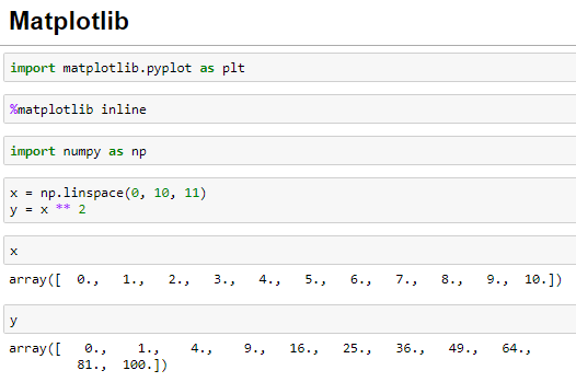
Let's first import the Matplotlib library and also recreate the NumPy Array we created in the previous post as the data for the plots. I suggest you to go through this post if you find any difficulties in any of the statements executed below:

Let's now create some plots with the Matplotlib:

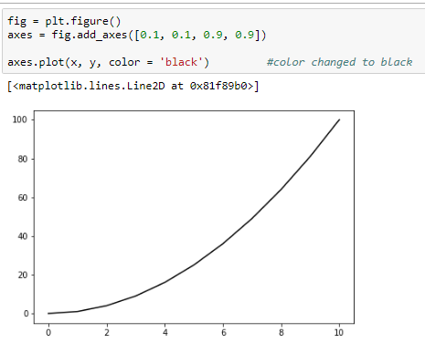
Change the plot color

Matplotlib supports two ways (using the color name and the RGB hex code) of changing the color of the plot using the color parameter of the plot method. I have changed the plot color to black using these two ways in the below example:

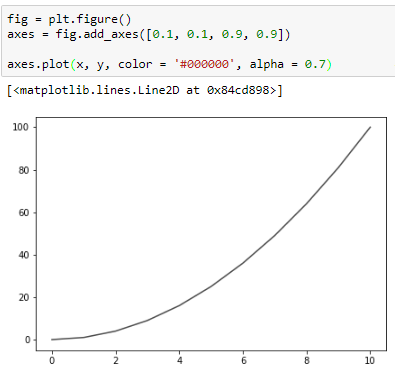
Change the line opacity

We can also change the opacity of the line of the plot using the alpha parameter of the plot method. The higher the alpha value the more opaque the plot. I have set the opacity to 0.8 in the below example:

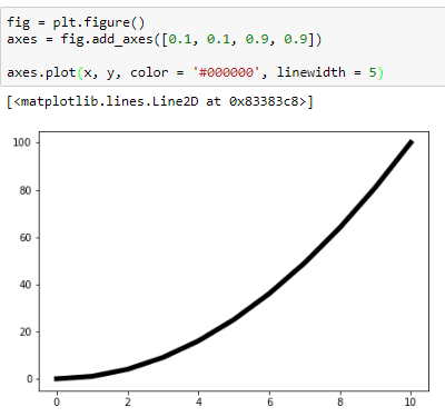
Change the line width

We can change the width of the line of the plot using the linewidth parameter of the plot method. I have changed the linewidth to five times the default line width in the below example:

Change the line style

Matplotlib also supports various line styles for the plots. These can be changed by the linestyle parameter of the plot method. Below is an example of the dashed line style supported by the plot method:

Here is a list of all the style types supported by the plot method:

['solid' | 'dashed' | 'dashdot' | 'dotted' | (offset, on-off-dash-seq) | '-' | '--' | '-.' | ':' | 'None' | ' ' | '']

Marker for the actual points

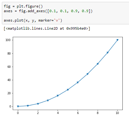
Matplotlib also supports marking actual points on the graph using the marker parameter of the plot() method. Here is an example of triangle down marker:

The following link lists all the marker types supported by the plot method. I also recommend visiting this awesome link which provides tons of other customization options we can do with Matplotlib. With this, we end this post on Matplotlib. From the next post onward, we'll learn about Seaborn, another very important Data Science library to plot beautiful statistical plots.

Xtensor & Xtensor-blas Library - Numpy for C++

Sahil Dadia CPP, data science, numpy, python, Tensor 3 comments

Xtensor & Xtensor-blas Library - Numpy for C++

Intro - What & Why?

I am currently working on my own deep learning & optimization library in C++, for my research in Data Science and Analytics Course at Maynooth University, Ireland. While searching for an existing tensor library (eigen/armadillo/trilinos - do not support tensors). I discovered Xtensor and Xtensor-blas, which has syntax like numpy and is avaliable for for C++ and Python.

Capabilities/Advantages (Xtensor to Numpy cheatsheet)

Numpy Like Syntax

typedef xt::xarray<double> dtensor;

dtensor arr1 {{1.0, 2.0, 3.0},   {2.0, 5.0, 7.0},   {2.0, 5.0, 7.0}}; // 2d array of double

dtensor arr2 {5.0, 6.0, 7.0}; // 1d array of doubles

cout << arr2 << "\n"; // outputs : {5.0, 6.0, 7.0}

Intuitive Syntax For Operation

typedef xt::xarray<double> dtensor;

dtensor arr1 {{1.0, 2.0, 3.0},   {2.0, 5.0, 7.0},   {2.0, 5.0, 7.0}}; // 2d array of double

dtensor arr2 {5.0, 6.0, 7.0}; // 1d array of doubles

cout << arr2 << "\n"; // outputs : {5.0, 6.0, 7.0}

// Reshape
arr1.reshape({1, 9});
arr2.reshape({1,9});
cout << arr1 << "\n"; // outputs : {1.0, 2.0, 3.0, 2.0, 5.0, 7.0, 2.0, 3.0, 7.0}

// Addition, Subtraction, Multiplication, Division
dtensor arr3 = arr1 + arr2;
dtensor arr3 = arr1 - arr2;
dtensor arr3 = arr1 * arr2;
dtensor arr3 = arr1 / arr2;

// Logical Operations
dtensor filtered_out = xt::where(a > 5, a, b);
dtensor var = xt::where(a > 5);
dtensor logical_and = a && b;
dtensor var = xt::equal(a, b);

// Random numbers
dtensor random_seed = xt::random::seed(0);
dtensor random_ints = xt::random::randint<int>({10, 10});

// Basic operations
dtensor summation_of_a = xt::sum(a);
dtensor mean = xt::mean(a);
dtensor abs_vals = xt::abs(a);
dtensor clipped_vals = xt::clip(a, min, max);

// Exponential & Power Functions
dtensor exp_of_a = xt::exp(a);
dtensor log_of_a = xt::log(a);
dtensor a_raise_to_b = xt::pow(a, b);

Easy Linear Algebra

// Vector product
dtensor dot_product = xt::linalg::dot(a, b)
dtensor outer_product = xt::linalg::outer(a, b)

// Inverse & solving system of equation
xt::linalg::inv(a)
xt::linalg::pinv(a)
xt::linalg::solve(A, b)
xt::linalg::lstsq(A, b)

// Decomposition
dtensor SVD_of_a = xt::linalg::svd(a)

// Norms & determinants
dtensor matrix_norm = xt::linalg::norm(a, 2)
dtensor matrix_determinant = xt::linalg::det(a)

Installation

Install Xtensor

cd ~ ; git clone https://github.com/QuantStack/xtensor
cd xtensor; mkdir build && cd build;
cmake -DBUILD_TESTS=ON -DDOWNLOAD_GTEST=ON ..
make
sudo make install

Install xtensor-blas

cd ~ ; git clone https://github.com/QuantStack/xtensor-blas
cd xtensor-blas; mkdir build && cd build;
cmake ..
make
sudo make install

Use In Your Code

It is a header only library


#include <xtensor/xarray.hpp>


#include <xtensor/xio.hpp>


#include <xtensor/xtensor.hpp>

Linking & Compilation flags
```
g++ -std=c++14 ./myprog.cpp -lblas
```

Where have I used it?

As mentioned in the intro, Xtensor and Xtensor-blas are the core component on which I have built my own deep learning & optimization library. This library is a monumental shift in C++ and ease of computation. In upcoming series of posts I will show you how to create your own library using xtensor.

In the next post, I will give an overview of the architecture of the project for your own library. And alongside I will introduce blas routines.

Data Science & Machine Learning - 6.3 Matplotlib Subplots & Other Features

Krishna Chaurasia data science, machine learning, matplotlib, python 3 comments

Hi friends,

Welcome to another post on Python's Matplotlib library under Data Science & Machine Learning. In the previous post, we discussed basic ways to draw plots using Matplotlib. In this post, we'll see how to draw subplots using the Matplotlib library.

Note: All the commands discussed below are run in the Jupyter Notebook environment. See this post on Jupyter Notebook to know about it in detail.

Matplotlib subplots

Let's first import the Matplotlib library and also recreate the NumPy Array we created in the previous post as the data for the plots. I suggest you to go through the previous post if you find any difficulties in any of the statements executed below:

Let's now start with the Matplotlib subplots. To create the Matplotlib subplots, the Matplotlib library provides the subplots() method:

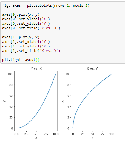
In the above figure, we can see that the subplots() method creates a figure and a set of subplots and the number of subplots are specified by the nrows and the ncols parameters (by default, their values are 1). Let's now create a subplot of one row and two columns using the subplots() method:

The plt.subplots() method itself adds the axes to the figure based on the nrows and the ncols values which were earlier required to be added manually by us in case of single plots in the previous post.

Further note that the axes variable in the above figure is an array of axes which is verified below:

Now, we can draw some plots using the NumPy Arrays we created above for each of the axes using the array indexing notation:

We can also add further customization(x-label, y-label, title) to each of the subplots just like we did in the previous post:

The tight_layout() method is used to avoid any overlap of values between the subplots.

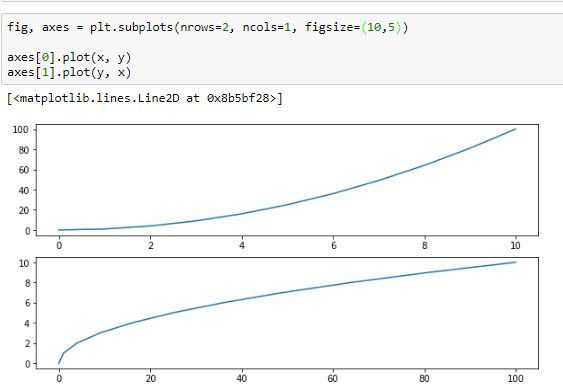
We can also change the size of the plots using figsize parameter. Here is an example:

Saving a Matplotlib plot

We can save a Matplotlib plot using the savefig() method passing the file name with the extension into a variety high quality formats such as png, jpeg, eps, pdf and many more.

And here is my jpeg file image:

You can also save the image as a pdf by passing the .pdf as extension:

We can also add legend to the figure using the legend() method in order to distinguish the plots. Here is the step to add the legend:

Remember to set the label parameter with each of the plots separately in order for the legend to work correctly.

We will end this post here on Matplotlib. In the next post, we will see various customization that can be done with the plots such as changing the line color, line width, line style and so on.

Data Science & Machine Learning - 6.2 Matplotlib Basic Plots

Krishna Chaurasia data science, machine learning, matplotlib, python 1 comment

Hi friends,

Welcome to another post on Matplotlib under Data Science & Machine Learning. In the previous post, we discussed the installation process of Matplotlib. In this we will see the basic plots supported by Matplotlib.

Note: All the commands discussed below are run in the Jupyter Notebook environment. See this post on Jupyter Notebook to know about it in detail.

Matplotlib Basic Plots

Before we can begin to use the Matplotlib library, we need to import it using the following command:

Although this will import the Matplotlib library in Python yet we need to run the following additional command in order for the plots to be displayed inside the Jupyter Notebook:

%matplotlib inline

This requests the Jupyter Notebook to display the plots inline i.e. within the Jupyter Notebook.

First, I have generated a NumPy Array of random numbers using the linspace method which will be used to draw the plots.

Let's now draw some plots using the Matplotlib library.

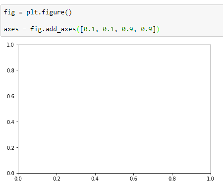
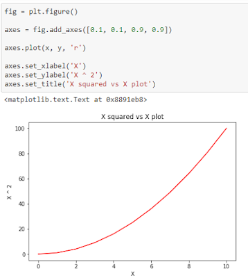
In the above figure, we have created a figure object (fig) using figure() method which renders a FigureCanvas (an empty background) to draw plots on using the Matplotlib library. Next, we add axes to the fig object created above using the add_axes() method:

The add_axes() method takes a list (with four elements) as a parameter signifying the left point, the bottom point, the width and the height respectively of the axes. You can pass in any values within the range [0, 1] for each of the parameters.

Next, we plot the above generated NumPy arrays on our axes using the plot() method:

Now, we can do several customization to our plot such as adding x and y labels, adding the plot title or changing the plot color:

We can also add multiple axes to the same plot. Here is an example of two axes within a figure object:

We can do similar customization as before by calling the required method on the appropriate axis object as shown below:

I have only discussed the object-oriented way of using Matplotlib here. You can also use the Matplotlib using the functional method by going through this official documentation. I however like the object-oriented way better since it provides flexibility and controlled way of usage. In the next post, we will discuss how to draw subplots inside the figure canvas and other advance features of Matplotlib library.

101. Symmetric Tree

Krishna Chaurasia geeksforgeeks, interview, interviewbit, leetcode, programming 1 comment

Given a binary tree, check whether it is a mirror of itself (ie, symmetric around its center).

For example, this binary tree [1,2,2,3,4,4,3] is symmetric:

But the following [1,2,2,null,3,null,3] is not:

Approach : Use the simple recursive solution.

/**
 * Definition for a binary tree node.
 * struct TreeNode {
 *     int val;
 *     struct TreeNode *left;
 *     struct TreeNode *right;
 * };
 */
bool checkIfSymmetric(struct TreeNode* n1, struct TreeNode* n2){
    if(n1 == NULL && n2 == NULL)
        return true;
    if(n1 == NULL || n2 == NULL)
        return false;
    
    if(n1->val == n2->val){
        return checkIfSymmetric(n1->left, n2->right) && checkIfSymmetric(n1->right, n2->left);
    }
    return false;
}
bool isSymmetric(struct TreeNode* root) {
   if(root == NULL){
       return true;
   }
   return checkIfSymmetric(root->left, root->right);
}

104. Maximum Depth of Binary Tree

Krishna Chaurasia binary tree, geeksforgeeks, leetcode, trees No comments

Given a binary tree, find its maximum depth. The maximum depth is the number of nodes along the longest path from the root node down to the farthest leaf node. Height of empty binary tree is 0 and with just root node is 1.

For the above example, the maximum depth is 3 following the path 1-2-5.

Approach : Using the recursive approach as implemented below.

/**
 * Definition for a binary tree node.
 * struct TreeNode {
 *     int val;
 *     struct TreeNode *left;
 *     struct TreeNode *right;
 * };
 */
int max(int a, int b){
    return a >= b ? a : b;
}
int maxDepth(struct TreeNode* root) {
    int height;
    //base case
    if(root == NULL){
        return 0;
    }
    //recursively compute left and right height and return the maximum
    height = 1 + max(maxDepth(root->left), maxDepth(root->right));
    return height;
}

83. Remove Duplicates from Sorted List

Krishna Chaurasia duplicate, geeksforgeeks, interviewbit, leetcode, linked list 1 comment

Given a sorted linked list, delete all duplicates such that each element appear only once.

For example,
Given 1->1->2, return 1->2.
Given 1->1->2->3->3, return 1->2->3.

Approach : The key to solve the problem is using the right loop condition and maintaining necessary pointers in each loop.

/**
 * Definition for singly-linked list.
 * struct ListNode {
 *     int val;
 *     struct ListNode *next;
 * };
 */
struct ListNode* deleteDuplicates(struct ListNode* head) {
    struct ListNode *cur, *_next;
    if(head == NULL || head->next == NULL){
        return head;
    }
    cur = head;
    while(cur && cur->next){
        //set the pointer of the current next to the next node if duplicate is found
        if(cur->val == cur->next->val){
            _next = cur->next->next;
            free(cur->next);
            cur->next = _next;
        }else{
            //else just move forward to next node
            cur = cur->next;
        }
    }
    return head;
}

100. Same Tree

Krishna Chaurasia binary tree, leetcode, trees 1 comment

Given two binary trees, write a function to check if they are equal or not.

Two binary trees are considered equal if they are structurally identical and the nodes have the same value.
Below are some examples:

Ex. 1:
Tree 1:
10
        20 30
40 50 60 70

Tree 2:
10
        20 30
40 50 60 70
Tree 1 & Tree 2 are identical.

Example 2:
Tree 1:
10
        20 30
40 50 60 70
Tree 2:
10
        20 30
40 60 50 70

Trees 1 & 2 are not identical as their structures are same but values at nodes 50 and 60 differ.

Example 3:
Tree 1:
10
20 30
40 50 60
Tree 2:
10
20 30
40 50 60

Trees 1 & 2 are not identical as the structures are not same as 60 is on left subtree of node 30 in Tree 1 but on right subtree of node 30 in Tree 2.

Approach : Use the simple recursive solution.

/**
 * Definition for a binary tree node.
 * struct TreeNode {
 *     int val;
 *     struct TreeNode *left;
 *     struct TreeNode *right;
 * };
 */
bool isSameTree(struct TreeNode* p, struct TreeNode* q) {
    if(p == NULL && q == NULL){
        return true;
    }
    if(p == NULL && q != NULL || p != NULL && q == NULL){
        return false;
    }
    if(p->val == q->val){
        return isSameTree(p->left, q->left) && isSameTree(p->right, q->right);
    }
    return false;
}

70. Climbing Stairs

Krishna Chaurasia geeksforgeeks, interview, leetcode, programming 1 comment

You are climbing a stair case. It takes n steps to reach to the top.

Each time you can either climb 1 or 2 steps. In how many distinct ways can you climb to the top?

Note: Given n will be a positive integer.

Approach : The standard recursive solution times out so the idea is to use the iterative solution to find the nth fibonacci number.

int climbStairs(int n) {
    int f1 = 2;
    int f2 = 1;
    if(n == 1) {
        return f2;
    } else if(n == 2) {
        return f1;
    }

    int fn;
    for(int i = 3; i <= n; i++) {
        fn = f1 + f2;
        f2 = f1;
        f1 = fn;
    }
    return fn;
}

Here is the link to the ideone solution : http://ideone.com/ErEU6E

69. Sqrt(x)

Krishna Chaurasia binary search, geeksforgeeks, interviewbit, leetcode No comments

Implement int sqrt(int x).

Return the floor if x is not a perfect square.

Approach : Using binary search making sure that overflow does not happen by taking long long.

class Solution {
public:
    int mySqrt(int x) {
        if(x <= 1){
      return x;
 }
     int low = 0, high = x / 2;
     //long to prevent overflow
 long long mid;
 while(low <= high){
     mid = (low + high) / 2;
     //needs to be long to prevent overflow
     long long t = mid * mid;
     //second part is to return floor if x is not perfect square
     if( t == x || ((t < x) && ((mid + 1) * (mid + 1) > x))){
      break;
     } else if(x < t){
      high = mid - 1;
     }else{
      low = mid + 1;
     }
 }
 return mid;
    }
};

Here is the link to the ideone solution : http://ideone.com/taTCKu

38. Count and Say

Krishna Chaurasia interview, leetcode, programming 1 comment

Problem: The count-and-say sequence is the sequence of integers with the first five terms as following:


1.     1

2.     11
3.     21

4.     1211

5.     111221

1 is read off as "one 1" or 11.


11 is read off as "two 1s" or 21.


21 is read off as "one 2, then one 1" or 1211.

Given an integer n, generate the nth term of the count-and-say sequence.

Note: Each term of the sequence of integers will be represented as a string.

Example 1:


Input: 1

Output: "1"

Example 2:


Input: 4

Output: "1211"

Approach: The solution is straight forward. The appendNext method is run over n times where n is the input.

class Solution {
public:
    public:
 
    string appendNext(string str){
        string str1;
        char ch = str[0];
        int chCount = 1;
        for(int i = 1; i <= str.size(); i++){
            if (str[i] == ch){
                chCount++;
            }
            else {
                char chr = chCount + '0';
                str1 = str1 + chr;
                str1 = str1 + ch;
                ch = str[i];
                chCount = 1;
            }
        }
        return str1;
    }
    
    string countAndSay(int n) {
        if (n == 1) {
            return "1";
        }
        string str1 = "1";
        string strn;
        for (int i = 1; i < n; i++){
            strn = appendNext(str1);
            str1 = strn;
        }
        return strn;
    }
};

Here is the link to the ideone solution : http://ideone.com/tbYXUM

Saturday, 21 October 2017

Sunday, 15 October 2017

Monday, 11 September 2017

Matplotlib Plots Customization

Change the plot color

Change the line opacity

Change the line width

Change the line style

Marker for the actual points

Saturday, 19 August 2017

Xtensor & Xtensor-blas Library - Numpy for C++

Intro - What & Why?

Capabilities/Advantages (Xtensor to Numpy cheatsheet)

Numpy Like Syntax

Intuitive Syntax For Operation

Easy Linear Algebra

Installation

Use In Your Code

Where have I used it?

Next Post

Matplotlib subplots

Saving a Matplotlib plot

Thursday, 17 August 2017

Matplotlib Basic Plots

Sunday, 13 August 2017

Saturday, 12 August 2017

Friday, 11 August 2017

Tuesday, 8 August 2017

Contact Me

Popular Posts

Categories

Blog Archive