67. Add Binary

Given two binary strings, return their sum (also a binary string).

For example,
a = "11"
b = "1"
Return "100"

Approach : The idea is to start from the right and keep adding digits and forwarding carry (if any). Also, take care of the case when one of them gets exhausted. For that, keep adding zero to the other one and forward carry if required. 

1 2 3 4 5 6 7 8 9 10 11 12 13 14 15 16 17 18 19 20 21 22 23 24 25 26 27 28 29 30 31 32 33 34 35 36 37 38 39 40 41 42 43 44 45 46 47

string Solution::addBinary(string a, string b) { int lenA = a.length(), lenB = b.length(); int i = lenA - 1, j = lenB - 1; int carry = 0; stack<char> out; int sum = 0; while(i >= 0 || j >= 0){ if(i >= 0 && j >= 0){ //convert to int and add sum = a[i] - '0' + b[j] - '0' + carry; i--; j--; } else{ //string a is exhausted if(i < 0){ sum = b[j] - '0' + carry; j--; } //string b is exhausted else{ sum = a[i] - '0' + carry; i--; } } //setting the carry accordingly if(sum > 1){ carry = 1; }else{ carry = 0; } sum = sum % 2; //convert back to character char aChar = '0' + sum; out.push(aChar); } //for final carry if(carry){ out.push('1'); } string res = ""; //reverse the output while(!out.empty()){ res = res + out.top(); out.pop(); } return res; }

Here is the link to the ideone solution : http://ideone.com/o5r3Eq

Read More

Data Science & Machine Learning - 6.1 Matplotlib & Its Installation

Hi friends,

Welcome to this post on Data Visualization under Data Science & Machine Learning. In the previous post, we performed some practical data analysis using Pandas on the Kaggle SF Salaries Dataset. In this post, we'll learn about Matplotlib, one of the most popular Python libraries for visualizing our results using various plots. 

About Matplotlib [1]

1. Matplotlib is a Python 2D plotting library which produces high quality figures in a variety of hardcopy formats and interactive environments across platforms
2. It allows us to generate plots directly from NumPy Arrays and Pandas DataFrames which makes it even more popular
3. It can be used in Python scripts, the Python and IPython shell, the jupyter notebook, web application servers, etc.
4. It is widely said that Matplotlib tries to make easy things easy and hard things possible

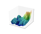
Here are some of the plots supported by the Matplotlib library:

Image source: Matlplotlib

Matplotlib Installation

Just like the installation of other Python libraries such as NumPy/Pandas, it is recommended to use the Anaconda distribution of Python in order to install Matlplotlib as well. You can see the installation of Anaconda distribution of Python here. Once you have that installed, you can install Matplotlib by running the following command in the command prompt:

conda install matplotlib

You can still install Matplotlib even if you don't have the recommended Anaconda distribution of Python (not recommended) using the following command:

pip install matplotlib

You can see the list of various plots supported by Matplotlib from this link. Now that we have installed Matplotlib successfully on our systems, we will start using the Matplotlib library starting with basic plots from the next post.

Read More

Data Science & Machine Learning - 5 SF Salaries Kaggle

Hi friends,

Welcome to another post under Data Science & Machine Learning. In the previous post, we discussed how to read and write data from and to various sources such as csv files, excel files, etc. using Pandas DataFrames. 

This post however will be different from the other ones in a way that we will not be learning anything new in this post but will be reviewing the concepts we have learnt till now using the SF Salaries Dataset available at the Kaggle website. Download the dataset from this Kaggle link. You will be required to login there in order to download the dataset. Once downloaded, copy and paste the csv file to your Jupyter Notebook. 

Note: All the commands discussed below are run in the Jupyter Notebook environment. See this post on Jupyter Notebook to know about it in detail. 

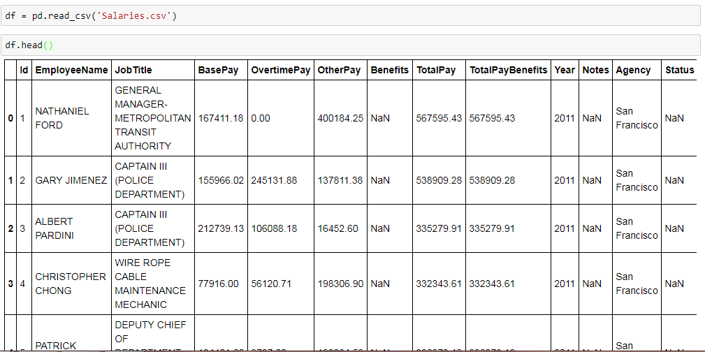
First, import the downloaded Salaries dataset using the read_csv method supported by the Pandas library:

Let's first see a few entries of the SF Salaries Dataset using the head method:

We can see that the dataset has the following columns:

1. Id
2. EmployeeName
3. JobTitle
4. BasePay
5. OvertimePay
6. OtherPay
7. Benefits
8. TotalPay
9. TotalPayBenefits
10. Year
11. Notes
12. Agency
13. Status

We can find the total number of entries in the SF dataset using the info method:

Now, let's answer some relevant questions using the concepts we have gathered till now:

1. Unique Job Titles in the dataset:





2. Top 10 most common Job Titles:





3. Average BasePay of the dataset:





4. Maximum amount of OvertimePay of the dataset:





5. JobTitle of ALBERT PARDINI:





6. TotalPayBenefits of ALBERT PARDINI:





7. Individual with highest TotalPayBenefits in the dataset: 




We can get the above result using the advance argmax method as well:





8. Average TotalPay year-wise:





9. Number of individuals with Chief in their Job Title: This involves lambda expression and might appear tricky at first sight but I suggest to break it down into sub steps for clear understanding. 

It is always advisable to explore various datasets from Kaggle or other websites since Data Science is not about just reading the theory but applying those concepts to datasets and gain insights to achieve a desirable output. From the next posts on ward, we'll start learning about another very important aspect of Data Science i.e. Data Visualizing. 

Read More

Data Science & Machine Learning - 4.7 Pandas Input Output

Hi friends,

Welcome to another post under Data Science & Machine Learning. In the previous post, we discussed various important methods supported by Pandas DataFrames. In this post, we will see another important feature of reading and writing data to and from Pandas DataFrames using various resources.

Note: All the commands discussed below are run in the Jupyter Notebook environment. See this post on Jupyter Notebook to know about it in detail. 

Pandas Input Output

To see the list of sources we can read data from into Pandas DataFrames, we type the pd.read_ in Jupyter Notebook and press Tab key. It shows the list of functions to read data from into the Pandas DataFrames.

Similarly, typing <df_name>.to_ and pressing the Tab key shows the list of functions to write data to various sources from a Pandas DataFrame.

Let's now see the usage of important ones.

1. Using CSV files: 
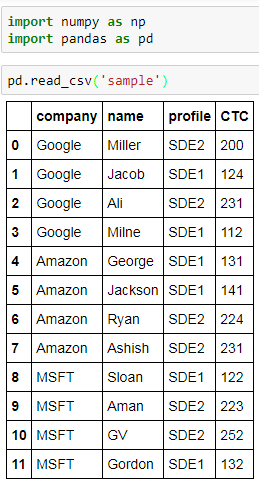
• The read_csv method is used to read data from csv files. Make sure that the csv file to be read from should be present in the current working directory. In the example below, I have a csv file named sample which I have read using the read_csv method.  





• The to_csv method on the other hand is used to write data to csv files.





2. Using Excel files: 


• The read_excel method is used to read data from Microsoft Excel files. Once again, make sure that the Excel file to be read from should be present in the current working directory. In the example below, I have an excel file named sample2 which I have read using the read_excel method.  





• The to_excel method on the other hand is used to write data from Pandas DataFrames to excel files





3. Using HTML files: 


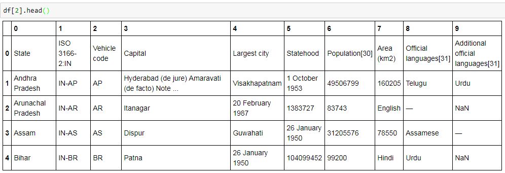
• We can even read data from a webpage provided it is contained within the table HTML tag. The read_html method is used to read data from tables in a webpage. Here is an example of read_html which reads data from the following Wikipedia URL.  





There are nine tables in the given Wikipedia URL which can be found by checking the length of the df variable





We can view each of them by using the access mechanism as in case of Python Lists. For example, to view a portion of the third table, run the following command in a Jupyter Notebook cell:

We can also load data to a Pandas DataFrame from a sql file but I'll leave it to you guys in case you are interested. In the next post under Data Science & Machine Learning, we will use the concepts we have learnt till now to explore the Kaggle SF Salaries Dataset.

Read More

Data Science & Machine Learning - 4.6 Pandas DataFrames Methods

Hi friends,

In the previous post under Data Science & Machine Learning, we discussed SQL functionalities of groupby, join and so on supported by Pandas DataFrames. In this post, we will see some important methods supported by the Pandas library that can be performed on DataFrames.

Note: All the commands discussed below are run in the Jupyter Notebook environment. See this post on Jupyter Notebook to know about it in detail. 

Pandas DataFrames Methods

Let's create a sample DataFrame to work with.

Here, I have created a sample DataFrame about employee details. 

So, let's now discuss the important methods supported by the Pandas library. 

1. head() - Returns only the top few elements of the DataFrame to get an idea of how the data in the DataFrame looks like





2. unique() - Returns the array of unique elements in a particular DataFrame's column





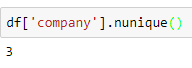
3. nunique() - Returns the number of unique elements in a particular DataFrame's column





4. value_counts() - Another very  important method that counts the occurrence of each element of a particular DataFrame column





5. apply() - Although we do have methods such as min, max, etc. supported by Pandas to work with DataFrames yet what if we want to apply custom methods to DataFrames? That's when the apply methods comes to the rescue. The apply method helps us apply our own user defined methods to a DataFrames' columns. So, let's see an example of the apply method:





In the above example, suppose we wanted to double the CTC of each employee of the DataFrame. For that, we have first defined our user defined method double and later use it on the CTC column using the apply method.

We can achieve the above result in a single step by using lambda expression as shown below:





6. columns() - Returns the list of column names of the DataFrame





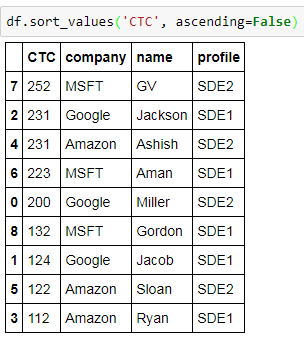
7. sort_values() - Sorts the DataFrame based on a specific column





We can also sort the DataFrame in descending order by setting the ascending parameter to False.

We end this post here but you can refer this link to get the complete list of methods supported by Pandas library. In the next post, we'll see the various ways to input and output data to and from the Pandas DataFrames.

Read More